osxQ Documentation
Designed for single‑machine research on Apple Silicon, osxQ combines a Python‑first workflow with MLX acceleration and unified memory to run mid‑scale state‑vector circuits — no CUDA required. Validation spans parity with PennyLane, Qulacs, and cuQuantum plus a QASMBench‑style OpenQASM 2.0 suite and a 200+ test corpus with circuit drawings (ASCII/Matplotlib/Quantikz). These docs cover install, the device‑style API, measurement modes (exact vs shot‑based), the reproducibility harness, scaling knobs, and curriculum‑ready examples.
Highlights
Overview
—For Apple Silicon systems, there has been no comprehensive, CUDA‑free, Apple‑native simulator mapping community benchmarks and OpenQASM suites directly to the platform. osxQ closes this gap. It is a Python‑first, MLX‑accelerated, Apple‑Silicon‑native state‑vector/MPS simulator targeting Metal unified memory (128–512 GB) to run mid‑scale circuits on a single machine — without shader programming or host‑device copy overhead.
osxQ reproduces community benchmarks (Yao.jl, PennyLane, Qulacs), provides parity with NVIDIA cuQuantum (cuStateVec), and runs a QASMBench‑style OpenQASM 2.0 suite. The library includes circuit drawing (ASCII, Matplotlib, Quantikz), exact and shot‑based measurement, and 200+ executable tests with analytical checks — mirroring pen‑and‑paper derivations with working code.
Backends & Architecture
- SV — Dense state‑vector simulator with device‑style API, sampling, and OpenQASM execution.
- MPS — Matrix Product State engine with two‑site SVD, truncation (
dmax,eps), non‑adjacent gates via swap‑network, and per‑run bond CSVs. - MPSD — MPS with TEBD‑optimized diagonal ZZ‑MPO (and optional pair‑sweeps). Produces distinct
_mpsdoutputs for clean comparison to MPS.
Why compare MPS vs MPSD? It isolates TEBD optimization effects, validates accuracy, reveals bond‑growth/truncation behavior, and guides defaults (dmax, eps, sweeps). Ablations become figure‑ready.
Paper Parity
To mirror the schedules used in “Comparative Benchmarking of Utility‑Scale Quantum Emulators” (arXiv:2504.14027), enable the preset which applies a quasi‑logarithmic qubit grid to the supported keys. All plots standardize the x‑axis label to Qubits.
# Apply paper‑2504 schedule (4,8,16,24,32,64,128,256; 512/1024 if cap allows)
./bench_with_logging.sh --paper-2504 --with-mps --with-mpsd --mps-dmax 128 --mps-eps 1e-10

# One‑off example
./bench.sh --paper-2504 --circuit qft --simulate-limit 256
Supported keys include: ghz, wstate, qft, qft_entangled/qftentangled, graph_state/graphstate, phase_estimation/qpeexact, phase_estimation_inexact/qpeinexact, ae, quantum_walk/quantum_walk_vchain/qwalk, random/random_circuit, realamp, su2rand, qnn.
Backends & Flags
# Backend selection
MLXQ_BACKEND=sv|mps

# MPS tuning
MLXQ_MPS_DMAX=128          # bond cap (default 64)
MLXQ_MPS_EPS=1e-10         # truncation epsilon
MLXQ_MPS_EARLY_STOP_BMAX=0 # stop when D ≥ this (0=off)
MLXQ_MPS_STOP_ON_TRUNC=0   # stop when any truncation occurs
MLXQ_MPS_PAIR_SWEEPS=0     # even/odd pair sweeps in TEBD

# MPSD mode (MPS + ZZ‑MPO; distinct _mpsd outputs)
MLXQ_MPSD=1                # enables _mpsd suffix and captions
MLXQ_MPS_USE_MPO_ZZ=1      # diagonal ZZ‑MPO for TEBD
Use ./bench_with_logging.sh --with-mps --with-mpsd to run SV → MPS → MPSD and copy artifacts for papers. For one‑offs, set env vars and call ./bench.sh --circuit <key>.
Utilities & Reporting
# Overlay mlxQ vs external CSV (e.g., cuStateVec or TN)
python3 tools/overlay_compare.py \
  --ours bench/qft_mps_data.csv \
  --ext mimiq_qft.csv --ext-time-col seconds --ext-scale-ms 1000 \
  --label-ours "osxQ (M‑series)" --label-ext "External" \
  --out bench/qft_overlay.png

# Aggregate MPS summaries into a single report (JSON + Markdown)
python3 tools/mps_report.py --bench bench

# Track D‑growth vs TEBD steps for a single circuit (ad‑hoc)
PYTHONPATH=src python3 tools/mps_dgrowth.py \
  --circuit tfim --n 16 --steps 40 --dt 0.05 --dmax 128 --eps 1e-10 \
  --out bench --plot
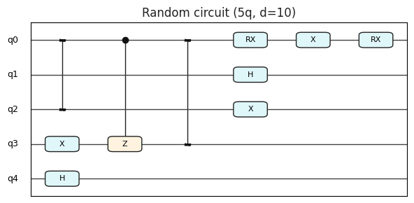
Screenshots & Circuit Gallery
rdcircuit001. Random/Yao‑style circuit used in visualization tests. Rounded corners for easy scanning.
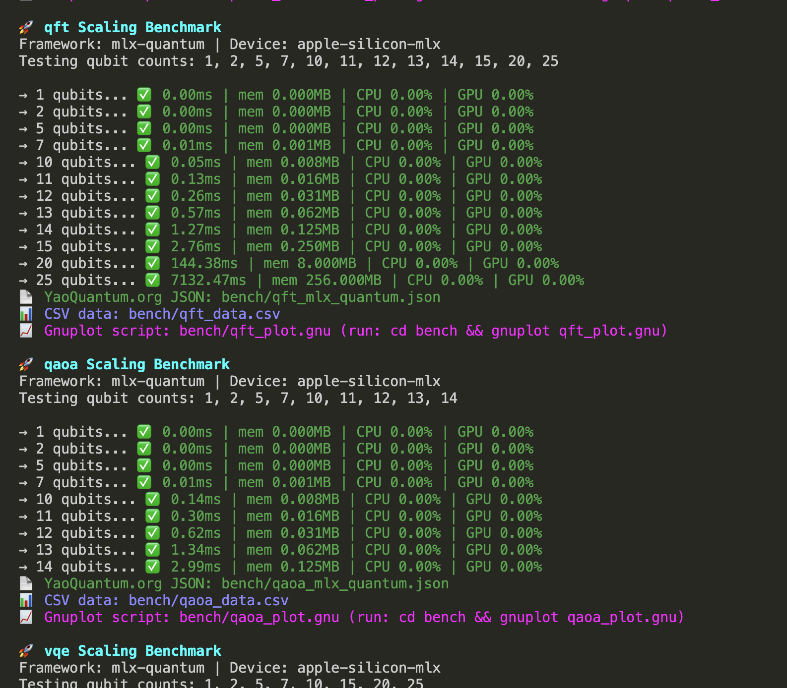
Algorithms & Benchmarks
Algorithm subjects
- QFT (Quantum Fourier Transform)
- Phase Estimation (PE)
- QAOA (Ising)
- VQE (Ising, UCCSD toy)
- Time Evolution / Trotterization
- Hamiltonian Simulation (toy Pauli models)
- Variational Circuit (ansatz sweep)
- GHZ, Grover, Random/Yao, QCBM, Steady State
Benchmark keys
- hamiltonian_simulation, time_evolution, trotter, steady_state
- random_circuit, qcbm, phase_estimation, qft
- qaoa, vqe, variational_circuit, grover, ghz
- cuquantum_blueqat (vendor parity)
MQTBench additions
- ghz, wstate, qft, qft_entangled/qftentangled
- qpeexact/qpeinexact, graph_state/graphstate, ae
- qwalk/quantum_walk_vchain, random/random_circuit
- realamp, su2rand, qnn
Many‑body variants
- TFIM (1st/2nd order), Heisenberg/XXZ (random field), long‑range Ising (1/rα), ladder Heisenberg (2×L)
Why compare MPS and MPSD?
- Performance: MPSD replaces dense 4×4 applies on ZZ with a diagonal MPO, reducing per‑bond cost in TEBD sweeps, especially at higher D.
- Parity: Both produce the same unitary; MPSD changes the kernel, not the model. JSON metadata includes
mps.mode(mpsormpsd). - Diagnostics: Bonds plots “flatten” once
Dmaxis reached. Increase--mps-dmaxand/or tighten--mps-epsto observe D‑growth.
Outputs
- Per‑bench CSV/JSON (scaling + hardware‑suffixed JSON)
- Per‑n bonds CSV (
<key>_mps[d]_n<N>_bonds.csv) and per‑bench summary (<key>_mps[d]_summary.csv) - Scaling and bond‑growth plots (
_scaling.png,_bonds.png) copied topaper/prx-quantum/images/andassets/benchmarks/
Vendor/framework groups
- Yao.jl (Random/Yao, QFT, time evolution)
- PennyLane (VQE, QAOA, circuit parity & drawing)
- Qulacs (reference workloads)
- NVIDIA cuQuantum (cuStateVec samples; Blueqat‑style brickwork)
Installation
Requirements: macOS 13.3+, Apple Silicon (M‑series), Python 3.11+, MLX.
python3 -m venv .venv
source .venv/bin/activate
python3 -m pip install --upgrade pip
python3 -m pip install mlx matplotlib
Quick Start
# Run validation tests (pretty output)
export PYTHONPATH=src
export MLXQ_PRINT_ASCII=1   # optional
python3 src/tests/run_core_tests.py

# Run algorithm benchmarks (saves plots)
export PYTHONPATH=src
python3 src/benchmark/bench.py

# Textual TUI (optional)
python3 -m pip install textual
python3 src/benchmark/bench_tui.py
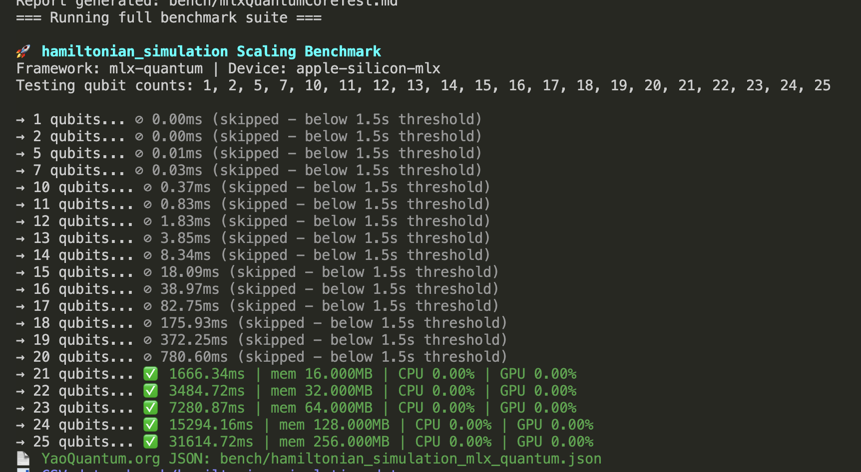
Sample Run
A single‑circuit scaling run of hamiltonian_simulation (cap 30; qubits 1→28). Rendered as a terminal snippet for clarity.
=== Running: ./bench.sh --circuit hamiltonian_simulation --simulate-limit 30 --qubits 1,2,5,7,10,11,12,13,14,15,16,17,18,19,20,21,22,23,24,25,26,27,28
=== Single-circuit run: hamiltonian_simulation (qubits: 1,2,5,7,10,11,12,13,14,15,16,17,18,19,20,21,22,23,24,25,26,27,28, cap: 30) ===
=== Running hamiltonian_simulation (qubits: 1,2,5,7,10,11,12,13,14,15,16,17,18,19,20,21,22,23,24,25,26,27,28, cap: 30) ===
hamiltonian_simulation Scaling Benchmark
Framework: mlx–quantum | Device: apple–silicon–mlx
Testing qubit counts: 1, 2, 5, 7, 10, 11, 12, 13, 14, 15, 16, 17, 18, 19, 20,
21, 22, 23, 24, 25, 26, 27, 28
Hamiltonian: H = ∑ ZᵢZᵢ₊₁ + 0.5 ∑ Xᵢ (J=1.0, h=0.5)
hamiltonian_simulation |  1q | gates    20 | wall   12.13 ms
hamiltonian_simulation |  2q | gates    60 | wall   13.33 ms
hamiltonian_simulation |  5q | gates   180 | wall   21.64 ms
hamiltonian_simulation |  7q | gates   260 | wall   27.66 ms
hamiltonian_simulation | 10q | gates   380 | wall   46.08 ms
hamiltonian_simulation | 11q | gates   420 | wall   44.06 ms
hamiltonian_simulation | 12q | gates   460 | wall   50.35 ms
hamiltonian_simulation | 13q | gates   500 | wall   58.00 ms
hamiltonian_simulation | 14q | gates   540 | wall   57.36 ms
hamiltonian_simulation | 15q | gates   580 | wall   63.27 ms
hamiltonian_simulation | 16q | gates   620 | wall   86.08 ms
hamiltonian_simulation | 17q | gates   660 | wall  137.84 ms
hamiltonian_simulation | 18q | gates   700 | wall  248.51 ms
hamiltonian_simulation | 19q | gates   740 | wall  514.43 ms
hamiltonian_simulation | 20q | gates   780 | wall 1038.66 ms
hamiltonian_simulation | 21q | gates   820 | wall 2152.24 ms
hamiltonian_simulation | 22q | gates   860 | wall 4399.28 ms
hamiltonian_simulation | 23q | gates   900 | wall 9287.86 ms
OpenQASM Suite
Place circuits under datasets/qasm/local/. Control caps via environment variables.
Environment Variables
QASM_MAX_QUBITS · QASM_TIMEOUT_MS · QASM_SIMULATE_LIMIT
Bench Controls
MLXQ_MAX_QUBITS · MLXQ_CAP_QFT · MLXQ_CAP_VQE · MLXQ_CAP_PHASE_ESTIMATION
Algorithms
QFT, PE, VQE, QAOA, GHZ, Grover, Random/Yao, QCBM, Trotter, Time Evolution
API Sketch
Python examples live under src/mlxq and src/tests. A minimal device‑style workflow looks like:
from mlxq.device import Device
from mlxq.gates import H, CNOT, RX, MeasureZ

dev = Device(n_qubits=3)
dev.apply(H(0))
dev.apply(CNOT(0, 1))
dev.apply(RX(2, 0.2))

exp = dev.expectation([MeasureZ(0), MeasureZ(1)])
print(exp)
Get in touch
Questions about osxQ, integrations, or research use? Reach out.